DATA-BASE (Oracle -9i /10c)

                                                            EF CODD’S 12 RULES

The relational data model was first developed by Dr. E.F. Codd, an IBM researcher, in 1970. In 1985, Dr. Codd published a list of 12 rules that concisely defined an ideal relational database. These rules have been used as a guideline for the design of all relational database systems since then.
I use the term "guideline" because, to date, no commercial relational database system fully conforms to all 12 rules. They do represent the relational ideal, though.

RULE 1: THE INFORMATION RULE
All data should be presented to the user in table form.

RULE 2: GUARANTEED ACCESS RULE
All data should be accessible without ambiguity. This can be accomplished through a combination of the table name, primary key, and column name.

RULE 3: SYSTEMATIC TREATMENT OF NULL VALUES
A field should be allowed to remain empty. This involves the support of a null value which is distinct from an empty string or a number with a value of zero. Of course, this can't apply to primary keys. Also, most database implementations support the concept of a nun-null field constraint that prevents null values in a specific table column.

RULE 4: DYNAMIC ON-LINE CATALOG BASED ON THE RELATIONAL MODEL
A relational database must provide access to its structure through the same tools that are used to access the data. This is usually accomplished by storing the structure definition within special system tables.

RULE 5: COMPREHENSIVE DATA SUBLANGUAGE RULE
The database must support at least one clearly defined language that includes functionality for data definition, data manipulation, data integrity, and database transaction control. All commercial relational databases use forms of the standard SQL (Structured Query Language) as their supported comprehensive language.

RULE 6: VIEW UPDATING RULE
Data can be presented to the user in different logical combinations, called views. Each view should support the same full range of data manipulation that direct access to a table has

RULE 7: HIGH-LEVEL INSERT, UPDATE, AND DELETE
Data can be retrieved from a relational database in sets constructed of data from multiple rows and/or multiple tables. This rule states that insert, update, and delete operations should be supported for any retrievable set rather than just for a single row in a single table.

RULE 8: PHYSICAL DATA INDEPENDENCE
The user is isolated from the physical method of storing and retrieving information from the database. Changes can be made to the underlying architecture (hardware, disk storage methods) without affecting how the user accesses it.

RULE 9: LOGICAL DATA INDEPENDENCE
How a user views data should not change when the logical structure (tables structure) of the database changes. This rule is particularly difficult to satisfy. Most databases rely on strong ties between the user view of the data and the actual structure of the underlying tables.

RULE 10: INTEGRITY INDEPENDENCE
The database language (like SQL) should support constraints on user input that maintain database integrity. This rule is not fully implemented by most major vendors. At a minimum, all databases do
Preserve two constraints through SQL.
•
No component of a primary key can have a null value. (see rule 3)
•
If a foreign key is defined in one table, any value in it must exist as a primary key in another table.

RULE 11: DISTRIBUTION INDEPENDENCE
A user should be totally unaware of whether or not the database is distributed (whether parts of the database exist in multiple locations). This is difficult to implement for a variety of reasons that we will
spend time on in future newsletters when we discuss distributed databases.

RULE 12: NONSUBVERSION RULE
There should be no way to modify the database structure other than through the multiple row database language (like SQL). Most databases today support administrative tools that allow some direct manipulation of the data structure.

Normalization of Database

Normalization rule are divided into following normal form.

1. First Normal Form           2  Second Normal Form
2. Third Normal Form          4 BCNF

First Normal Form (1NF)

As per First Normal Form, no two Rows of data must contain repeating group of information i.e each set of column must have a unique value, such that multiple columns cannot be used to fetch the same row. Each table should be organized into rows, and each row should have a primary key that distinguishes it as unique.

The Primary key is usually a single column, but sometimes more than one column can be combined to create a single primary key. For example consider a table which is not in First normal form

Student Table :

Student	Age	Subject
Adam	15	Biology, Maths
Alex	14	Maths
Stuart	17	Maths

In First Normal Form, any row must not have a column in which more than one value is saved, like separated with commas. Rather than that, we must separate such data into multiple rows.

Student Table following 1NF will be :

Student	Age	Subject
Adam	15	Biology
Adam	15	Maths
Alex	14	Maths
Stuart	17	Maths

Using the First Normal Form, data redundancy increases, as there will be many columns with same data in multiple rows but each row as a whole will be unique.

Second Normal Form (2NF)

As per the Second Normal Form there must not be any partial dependency of any column on primary key. It means that for a table that has concatenated primary key, each column in the table that is not part of the primary key must depend upon the entire concatenated key for its existence. If any column depends only on one part of the concatenated key, then the table fails Second normal form.

In example of First Normal Form there are two rows for Adam, to include multiple subjects that he has opted for. While this is searchable, and follows First normal form, it is an inefficient use of space. Also in the above Table in First Normal Form, while the candidate key is {Student, Subject}, Age of Student only depends on Student column, which is incorrect as per Second Normal Form. To achieve second normal form, it would be helpful to split out the subjects into an independent table, and match them up using the student names as foreign keys.

New Student Table following 2NF will be :

Student	Age
Adam	15
Alex	14
Stuart	17

In Student Table the candidate key will be Student column, because all other column i.e Age is dependent on it.

New Subject Table introduced for 2NF will be :

Student	Subject
Adam	Biology
Adam	Maths
Alex	Maths
Stuart	Maths

In Subject Table the candidate key will be {Student, Subject} column. Now, both the above tables qualifies for Second Normal Form and will never suffer from Update Anomalies. Although there are a few complex cases in which table in Second Normal Form suffers Update Anomalies, and to handle those scenarios Third Normal Form is there.

---

Third Normal Form (3NF)

Third Normal form applies that every non-prime attribute of table must be dependent on primary key, or we can say that, there should not be the case that a non-prime attribute is determined by another non-prime attribute. So this transitive functional dependency should be removed from the table and also the table must be in Second Normal form. For example, consider a table with following fields.

Student_Detail Table :

Student_id	Student_name	DOB	Street	city	State	Zip

In this table Student_id is Primary key, but street, city and state depends upon Zip. The dependency between zip and other fields is called transitive dependency. Hence to apply 3NF, we need to move the street, city and state to new table, with Zip as primary key.

New Student_Detail Table :

Student_id	Student_name	DOB	Zip

Address Table :

Zip	Street	city	state

---

The advantage of removing transtive dependency is,

• Amount of data duplication is reduced.
• Data integrity achieved.

---

Boyce and Codd Normal Form (BCNF)

Boyce and Codd Normal Form is a higher version of the Third Normal form. This form deals with certain type of anamoly that is not handled by 3NF. A 3NF table which does not have multiple overlapping candidate keys is said to be in BCNF. For a table to be in BCNF, following conditions must be satisfied:

• R must be in 3rd Normal Form
• and, for each functional dependency ( X -> Y ), X should be a super Key

E-R Diagram

ER-Diagram is a visual representation of data that describes how data is related to each other.

---

Symbols and Notations

---

Components of E-R Diagram

The E-R diagram has three main components.

1) Entity

An Entity can be any object, place, person or class. In E-R Diagram, an entity is represented using rectangles. Consider an example of an Organisation. Employee, Manager, Department, Product and many more can be taken as entities from an Organisation.

---

Weak Entity

Weak entity is an entity that depends on another entity. Weak entity doen't have key attribute of their own. Double rectangle represents weak entity.

.

---

2) Attribute

An Attribute describes a property or characterstic of an entity. For example, Name, Age, Address etc can be attributes of a Student. An attribute is represented using eclipse.

---

Key Attribute

Key attribute represents the main characterstic of an Entity. It is used to represent Primary key. Ellipse with underlying lines represent Key Attribute.

---

Composite Attribute

An attribute can also have their own attributes. These attributes are known as Composite attribute.

---

3) Relationship

A Relationship describes relations between entities. Relationship is represented using diamonds.

There are three types of relationship that exist between Entities.

• Binary Relationship
• Recursive Relationship
• Ternary Relationship

---

Binary Relationship

Binary Relationship means relation between two Entities. This is further divided into three types.

1. One to One : This type of relationship is rarely seen in real world.

The above example describes that one student can enroll only for one course and a course will also have only one Student. This is not what you will usually see in relationship.
2. One to Many : It reflects business rule that one entity is associated with many number of same entity. The example for this relation might sound a little weird, but this menas that one student can enroll to many courses, but one course will have one Student.

The arrows in the diagram describes that one student can enroll for only one course.
3. Many to One : It reflects business rule that many entities can be associated with just one entity. For example, Student enrolls for only one Course but a Course can have many Students.

4. Many to Many :

The above diagram represents that many students can enroll for more than one courses.

---

Recursive Relationship

When an Entity is related with itself it is known as Recursive Relationship.

---

Ternary Relationship

Relationship of degree three is called Ternary relationship.

Generalization

Generalization is a bottom-up approach in which two lower level entities combine to form a higher level entity. In generalization, the higher level entity can also combine with other lower level entity to make further higher level entity.

---

Specialization

Specialization is opposite to Generalization. It is a top-down approach in which one higher level entity can be broken down into two lower level entity. In specialization, some higher level entities may not have lower-level entity sets at all.

---

Aggregration

Aggregration is a process when relation between two entity is treated as a single entity. Here the relation between Center and Course, is acting as an Entity in relation with Visitor.

What is a KEY ?

A KEY  is a value used to uniquely identify a record in a table. A KEY could be a single column or combination of multiple columns

Note: Columns in a table that are NOT used to uniquely identify a record are called non-key columns.

What is a primary Key?

A primary is a single column values used to uniquely identify a database record. It has following attributes A primary key cannot be NULL A primary key value must be unique The primary key values can not be changed The primary key must be given a value when a new record is inserted.

What is a composite Key?

A composite key is a primary key composed of multiple columns used to identify a record uniquely

In our database , we have two people with the same name Robert Phil but they live at different places.

Hence we require both Full Name and Address to uniquely identify a record. This is a composite key.

Introducing Foreign Key!

In Table 2, Membership_ID is the foreign Key

Foreign Key references primary key of another Table!It helps connect your Tables A foreign key can have a different name from its primary key It ensures rows in one table have corresponding rows in another Unlike Primary key they do not have to be unique. Most often they aren't Foreign keys can be null even though primary keys can not

Why do you need a foreign key ?

Suppose an idiot inserts a record in Table B such as

You will only be able to insert values into your foreign key that exist in the unique key in the parent table. This helps in referential integrity. 

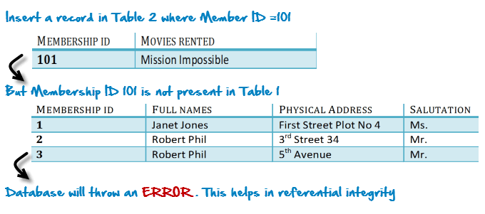
The above problem can be overcome by declaring membership id  from Table2  as foreign key of membership id  from Table1 

Now , if somebody tries to insert a value in the membership id  field that does not exist in the parent table , an error will be shown!

What is a transitive functional dependencies?

A transitive functional dependency is when changing a non-key column , might cause any of the other non-key columns to change

Consider the table 1. Changing the non-key column Full Name , may change Salutation.

Introduction to SQL

Structure Query Language(SQL) is a programming language used for storing and managing data in RDBMS. SQL was the first commercial language introduced for E.F Codd's Relational model. Today almost all RDBMS(MySql, Oracle, Infomix, Sybase, MS Access) uses SQL as the standard database language. SQL is used to perform all type of data operations in RDBMS.

---

SQL Command

SQL defines following data languages to manipulate data of RDBMS.

---

DDL : Data Definition Language

All DDL commands are auto-committed. That means it saves all the changes permanently in the database.

Command	Description
create	to create new table or database
alter	for alteration
truncate	delete data from table
drop	to drop a table
rename	to rename a table

DML : Data Manipulation Language

DML commands are not auto-committed. It means changes are not permanent to database, they can be rolled back.

Command	Description
insert	to insert a new row
update	to update existing row
delete	to delete a row
merge	merging two rows or two tables

---

TCL : Transaction Control Language

These commands are to keep a check on other commands and their affect on the database. These commands can annul changes made by other commands by rolling back to original state. It can also make changes permanent.

Command	Description
commit	to permanently save
rollback	to undo change
savepoint	to save te

DCL : Data Control Language

Data control language provides command to grant and take back authority.

Command	Description
grant	grant permission of right
revoke	take back permission.

---

DQL : Data Query Language

Command	Description
select	retrieve records from one or more table

create command

create is a DDL command used to create a table or a database.

---

Creating a Database

To create a database in RDBMS, create command is uses. Following is the Syntax,

create database database-name;

---

Example for Creating Database

create database Test;

The above command will create a database named Test.

---

Creating a Table

create command is also used to create a table. We can specify names and datatypes of various columns along.Following is the Syntax,

create table table-name
{
 column-name1 datatype1,
 column-name2 datatype2,
 column-name3 datatype3,
 column-name4 datatype4
};

Example for creating Table

create table Student(id int, name varchar, age int);

The above command will create a new table Student in database system with 3 columns, namely id, name and age.

alter command

alter command is used for alteration of table structures. There are various uses of alter command, such as,

• to add a column to existing table
• to rename any existing column
• to change datatype of any column or to modify its size.
• alter is also used to drop a column.

---

To Add Column to existing Table

Using alter command we can add a column to an existing table. Following is the Syntax,

alter table table-name add(column-name datatype);

Here is an Example for this,

alter table Student add(address char); 

The above command will add a new column address to the Student table

---

To AddMultiple Column to existing Table

Using alter command we can even add multiple columns to an existing table. Following is the Syntax,

alter table table-name add(column-name1 datatype1, column-name2 datatype2, column-name3 datatype3);

Here is an Example for this,

alter table Student add(father-name varchar(60), mother-name varchar(60), dob date); 

The above command will add three new columns to the Student table

---

To Add column with Default Value

alter command can add a new column to an existing table with default values. Following is the Syntax,

alter table table-name add(column-name1 datatype1 default data);

Here is an Example for this,

alter table Student add(dob date default '1-Jan-99'); 

The above command will add a new column with default value to the Student table

---

To Modify an existing Column

alter command is used to modify data type of an existing column . Following is the Syntax,

alter table table-name modify(column-name datatype);

Here is an Example for this,

alter table Student modify(address varchar(30)); 

The above command will modify address column of the Student table

---

To Rename a column

Using alter command you can rename an existing column. Following is the Syntax,

alter table table-name rename old-column-name to column-name;

Here is an Example for this,

alter table Student rename address to Location; 

The above command will rename address column to Location.

---

To Drop a Column

alter command is also used to drop columns also. Following is the Syntax,

alter table table-name drop(column-name);

Here is an Example for this,

alter table Student drop(address); 

The above command will drop address column from the Student table

SQL queries to Truncate, Drop or Rename a Table

truncate command

truncate command removes all records from a table. But this command will not destroy the table's structure. When we apply truncate command on a table its Primary key is initialized. Following is its Syntax,

truncate table table-name

Here is an Example explaining it.

truncate table Student;

The above query will delete all the records of Student table.

truncate command is different from delete command. delete command will delete all the rows from a table whereas truncate command re-initializes a table(like a newly created table).

For eg. If you have a table with 10 rows and an auto_increment primary key, if you use delete command to delete all the rows, it will delete all the rows, but will not initialize the primary key, hence if you will insert any row after using delete command, the auto_increment primary key will start from 11. But in case of truncatecommand, primary key is re-initialized.

---

drop command

drop query completely removes a table from database. This command will also destroy the table structure. Following is its Syntax,

drop table table-name

Here is an Example explaining it.

drop table Student;

The above query will delete the Student table completely. It can also be used on Databases. For Example, to drop a database,

 drop database Test;

The above query will drop a database named Test from the system.

---

rename query

rename command is used to rename a table. Following is its Syntax,

rename table old-table-name to new-table-name

Here is an Example explaining it.

rename table Student to Student-record;

The above query will rename Student table to Student-record.

DML command

Data Manipulation Language (DML) statements are used for managing data in database. DML commands are not auto-committed. It means changes made by DML command are not permanent to database, it can be rolled back.

---

1) INSERT command

Insert command is used to insert data into a table. Following is its general syntax,

INSERT into table-name values(data1,data2,..)

Lets see an example,

Consider a table Student with following fields.

S_id	S_Name	age

INSERT into Student values(101,'Adam',15);

The above command will insert a record into Student table.

S_id	S_Name	age
101	Adam	15

---

Example to Insert NULL value to a column

Both the statements below will insert NULL value into age column of the Student table.

INSERT into Student(id,name) values(102,'Alex');

Or,

INSERT into Student values(102,'Alex',null);

The above command will insert only two column value other column is set to null.

S_id	S_Name	age
101	Adam	15
102	Alex

---

Example to Insert Default value to a column

INSERT into Student values(103,'Chris',default)

S_id	S_Name	age
101	Adam	15
102	Alex
103	chris	14

Suppose the age column of student table has default value of 14.

Also, if you run the below query, it will insert default value into the age column, whatever the default value may be.

INSERT into Student values(103,'Chris')

---

2) UPDATE command

Update command is used to update a row of a table. Following is its general syntax,

UPDATE table-name set column-name = value where condition;

Lets see an example,

update Student set age=18 where s_id=102;

S_id	S_Name	age
101	Adam	15
102	Alex	18
103	chris	14

---

Example to Update multiple columns

UPDATE Student set s_name='Abhi',age=17 where s_id=103; 

The above command will update two columns of a record.

S_id	S_Name	age
101	Adam	15
102	Alex	18
103	Abhi	17

---

3) Delete command

Delete command is used to delete data from a table. Delete command can also be used with condition to delete a particular row. Following is its general syntax,

DELETE from table-name;

---

Example to Delete all Records from a Table

DELETE from Student;

The above command will delete all the records from Student table.

---

Example to Delete a particular Record from a Table

Consider the following Student table

S_id	S_Name	age
101	Adam	15
102	Alex	18
103	Abhi	17

DELETE from Student where s_id=103;

The above command will delete the record where s_id is 103 from Student table.

S_id	S_Name	age
101	Adam	15
102	Alex	18